Parameter Scan
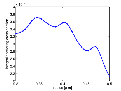
With the parameterization of the test project in the previous section Keyword Substitution, it is straightforward to run a parameter scan within Python:
1 2 3 4 5 6 7 8 9 10 11 12 13 14 15 16 17 18 19 20 21 22 23 24 25 26 27 28 29 30 | import jcmwave
import numpy as np
import os
# holds computed scattering cross sections
scattering_cross_section_scan = []
# loop over radius values
radii = np.linspace(0.3, 0.5, 40)
for radius in radii:
print ('Solving for radius %5.2e' %(radius,))
# set current parameter and solve the project
keys = {'radius': radius}
results = jcmwave.solve('mie2D.jcmp', keys=keys,
logfile=open(os.devnull, 'w'))
scs = results[1]['ElectromagneticFieldEnergyFlux'][0][0].real
# gather results
scattering_cross_section_scan.append(scs)
# plot scattering cross section against rod radius
from matplotlib.pyplot import *
plot(radii, scattering_cross_section_scan, '-+', linewidth=2, markersize=14)
xlabel('radius [$\mu$ m]', fontsize=14)
ylabel('integral scattering cross section', fontsize=14)
axis('tight')
show()
|
In line 6 we initialize the vector scattering_cross_section_scan which later holds the computed data. In line 9 we define an equidistant parameter sampling for the rod radius. In line 10 we start a loop over the sampling. In each step the dictionary keys is updated with the current radius value (line 14), followed by a solver call (line 15). The optional parameter logfile redirects the solver console output to a file (using os.devnull disregards all console output). In line 21 we gather the relevant data. Line 25-30 serve the plotting of the results, see Figure “Scattering Cross Section”.
The next section Python Code Snippets how to enrich the .jcmt input files with python scripts blocks.
